Airbnb Pricing Edinburgh
A link to the powerpoint for the project is provided here The Airbnb market has slowly taken over the touristy capital of Scotland and my home town Edinburgh. There are currently around 6000 properties in Edinburgh and I wanted to know, what dictates their price, is it just location…whether they are dog friendly or you can hold a party in them. More than just what features but how do the Airbnb rental prices relate to the average prices of houses in that area, is what home owners cherish in value the same as what a visitor looks for. There lies my hypothesis and prior bias, the features dictating a houses price are not fully correlated to what allows you to charge more for an Airbnb and therefore market opportunities exist for those wanting to purchase rental properties. So to achieve this I scraped Airbnb for 1600 property listings taking in all 44 features (ammenities, location…). On the otherside I scraped ESPC, for the price of the last 19 000 houses sold in Edinburgh over the last 2 years. I merged the data set so that each Airbnb was associated to the average house price in that area. After exploring the data I created a number of regression models which allowed me to get about a 70% prediction accuracy (to be improved).
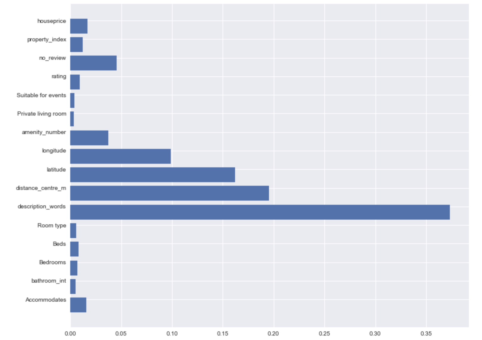
So the important features:
As I show in the plot below the most important features determining rental prices:
- Length of description (how many words), there is a major cutoff <100 words
- How many people your place accommodates (not how many rooms necessarily).
- Location, location, location! (This drives price greatly in particular distance to Princess st)
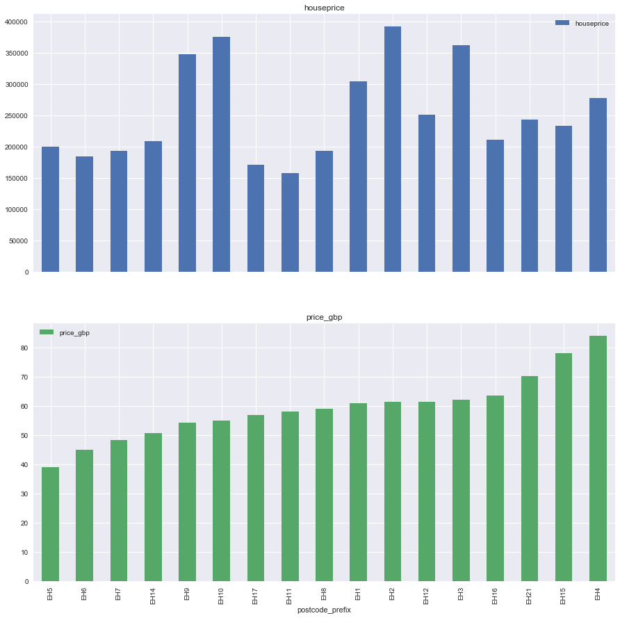
- Total number of amenities. But to the big question, there is not a major correlation to average area house prices and the rental price of the house, below I put the average house prices by postcode (241 kGBP for all of the EH’s) vs the average rental price of 60 GBP and we see that the places with the most expensive Airbnb rentals are places with average or below average house prices. In a separate post I detail the exploration of the Edinburgh housing market. Let’s break it down with an example (this is illustrative more than anything).
The Hypothesis
This all started with the concept that there existed opportunities in the Edinburgh marketplace for Airbnb rentals. Because the residential market is so dominated by pre-concieved notions of “areas” which are in-grained in the Edinburgh phyche, and therefore pay a premium for this commodity of living in the Grange or Murrayfield. However, for tourists there is no notion to THE areas, Edinburgh is not like the New York’s or London where even if you have never visited before, you are already aware of Manhattan the upper East side, Brooklyn… In fact my expectation is that the distance to the castle would be a determining factor in the price, and therefore, Grange (average house price=350 000 GBP) or Leith (average house price=190 000 GBP) would have the same value on the tourist market. Well there you go, my bias from 18 years of living in Edinburgh.
The Methodology
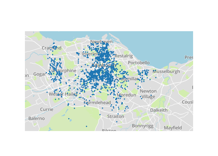
I managed to scrape the Airbnb website through a Python script, with the help of Selenium. Scraping the rental site’s page faced two major hurdles: 1) Airbnb have there own algorithm for presenting you properites, they pre-select a maximum of ~300 properties to present to you when you search a city. This means that you don’t get to see the full list of available properties in one go. To get around this I subdivided Edinburgh into quadrants which I searched and looped through individually grabbing all the properties in a small area of the city. Then I panned the map to pick up more and more properties. 2) Airbnb does not give the address of the properties, so I had to scrape the map and the tags for each property. These tags were relative positions in pixels which I then converted using the map anchors, esentially to top left and bottom right map position (NE+SW-Longitude/latitude positions of the map). From this
I was able to calculate the latitude and longitude of each property. From scraping the search page in addition to the individual property adverts I was able to accumulate up to about 44 features for each property (mainly) comprising of the amenities. In addition using GeoPy I was able to convert the latitudes and longitudes into an address with a postal code.
To evaluate the second objective of associating the house prices in Edinburgh, I scraped the ESPC realtor website, taking property details (price, address and property description) for the last 2 years of properties sold (approximately 19 500). This data was then aggregated and averaged by postcode in order to provide an additional feature in the Airbnb regression.
Before trying to regress on the data the number of features was reduced from 44 to 17. This was mainly achieved through combining all the various amenities into an amenity which was the sum of all the amenities which were given in the rental advertisement. In addition, for linear regression models, due to the large variation of magnitude in the features used, the values of the features was normalised.
In order to create models to predict the rental prices, various multi-linear regression models were initially used including the Lasso which provided some decent results outlined below. Finally a Gradient Boosted tree model was used with a depth of 4. Other decision tree and Random forest approaches were tried however, yielding poorer results with the data being susceptible to overfitting.
The tools used to achieve all this was Python with the following packages: Scikitlearn, GoePy, ML Insights and plot.ly.
What to take from it (results)
Data Exploration
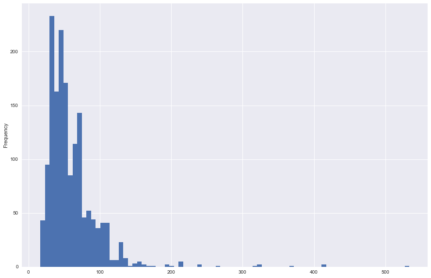
The table below outlines some key stats regarding the data set of rental prices, the mean rent in Edinburgh for the data collected was ~60 GBP. Also, the distribution of the data is as expected with a right skewed distribution, as seen with property prices. For the analysis, 4 properties which were more than 300 GBP were removed from the data.
| Parameter | Value (GBP) |
|---|---|
| Mean | 59.7 |
| Std. Deviation | 37.1 |
| Min | 16.67 |
| Max | 533.33 |
One key graphic in the exploration is a comparison of rental prices by postal code and the average house price in the area, as can be seen in the below graphic, there are no key correlation between the house price and the postal code, with the most expensive rental areas not being correlated to the most expensive housing areas.
Lasso Multi-linear Regression
The Lasso model was used as a progression onto the attempts with multi-linear regression, the parameters were normalised and in general the fit was moderate, with an R^{2} of 0.51 and a mean absolute deviation of 14.6 GBP. In general low cost rentals were well predicted but as we moved up the chain to more expensive properties it was clear that the model gave a poorer fit in part this can be attributed to the non-linearity in a lot of the features especially in the categorical features where we were representing house type as integer figures.
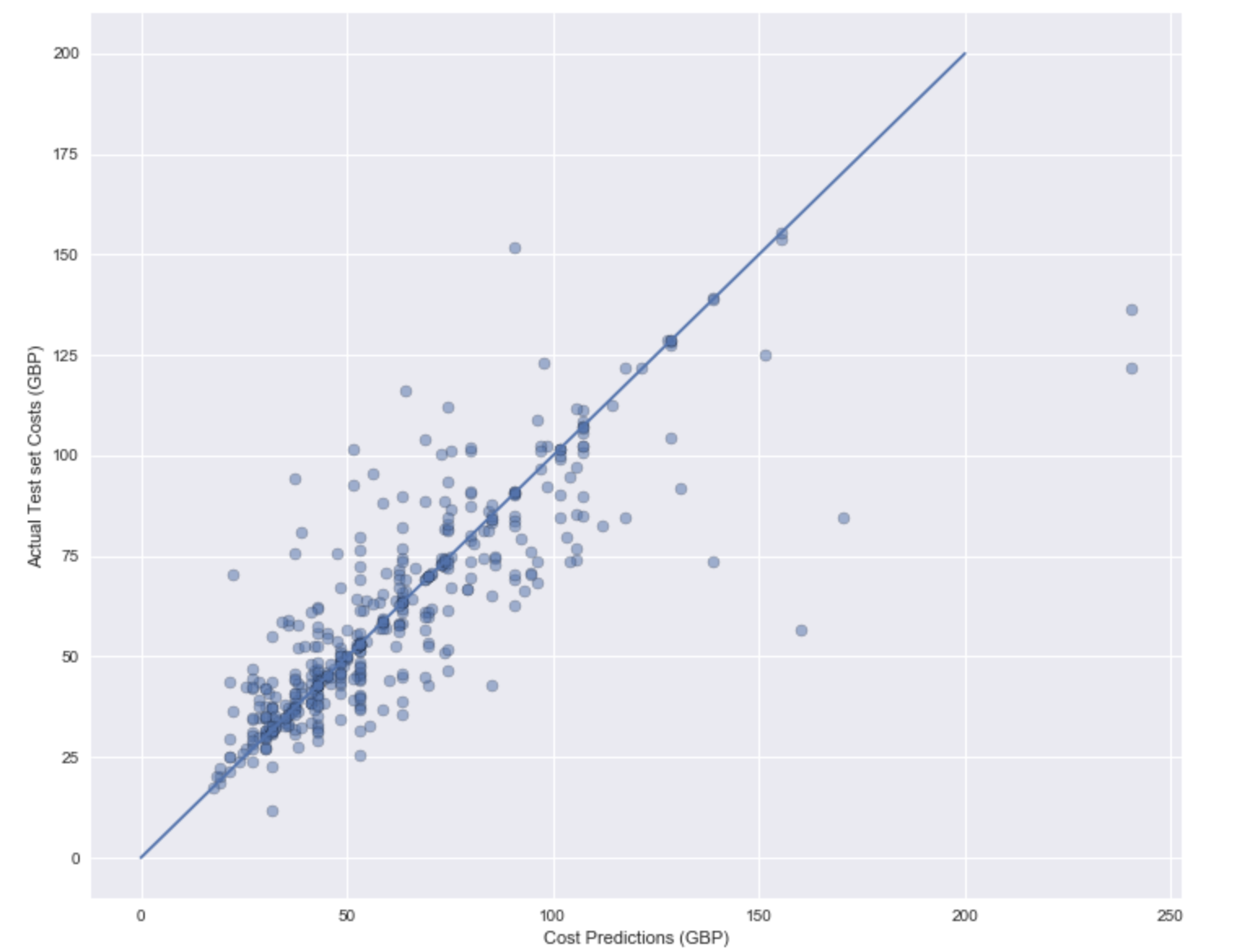
Gradient Boosted Tree
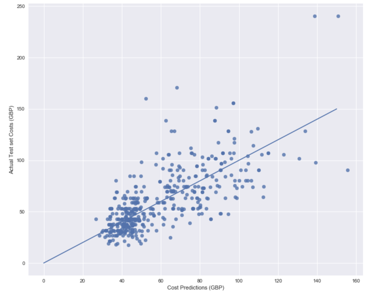
By far the best matches were achieved with gradient boosted trees, a depth of 4 was used, going to deeper trees began to overfit the data and there was poor performance exhibited in the test sets. Overall the model achieves an R^{2} of 0.7, the model suffers in price matching above the mean values, with the results being in generally under predicted. This is likely attributed to not having sufficient features representing the quality factor of each house. A further study should look to include indicators about the quality using reviews or photos in order to assist.
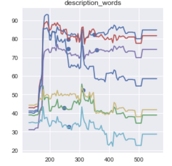
The most important factors was qualitatively the number of words in the description, however, as is shown in the below sensitivity plot, the importance of this was in general separating between advertisements with <100 words and after 100 words was written the benefit of additional words is stable. The other important factors was the location (here being distance to centre, longitude and latitude).
The below chart looks at varying the number of words in the description and the impact on the price, it can be seen that with all other parameters being equal in general the above 100 words there is little impact on price.
Further Work
The study will look to improve in the next stages by integrating content analysis for key words indicating the quality. This will also involve parsing the reviews to indicate the quality of the apartment. In addition, the data set will be increased trying to grab all available Airbnb’s in Edinburgh.
Thanks
A thanks to Brian Lucena and Andrew Blevins for their guidance.